Deimos' datastructures

We will now look at the basic data structures of Verdict and how exactly they are used in Deimos. Following this, we can understand how these data structures allow us to track provably correct behavior. We are talking about append-only hashchains and indexed Merkle trees.

Append-only hashchains

The paper does not describe an exact implementation of the hashchains, all we know is:

In Verdict’s transparency dictionary, the value associated with a label is an append-only hashchain of operations, where nodes store raw operations requested on the label, as well as the cryptographic hash of the previous node in the chain. For example, in the context of key transparency, a hashchain records two types of operations: (1) adding a new key; and (2) revoking an existing key [...]

So a conceivable implementation of each Hashchain element could include the following values:

• hash: the following three elements are hashed in a hash function and the value is stored in this field
• previous hash: a unique reference to the previous entry in the list, which depends on the contents of the entry as it contains the hashed values.
• operation: The executed operation, in our concrete application case ADD and REVOKE operations can be executed.
• value: Since we are still dealing with public keys, we need to know which keys are added or revoked in order to generate a list of valid, unrevoked keys from the operations.

Users can therefore register a unique ID in Deimos in the form of an e-mail address together with an initial public key. Any number of additional public keys can then be added, and keys that have already been added can be revoked. The prerequisite for adding new keys or revoking existing keys is that the operation has been signed with a private key associated with some unrevoked public key of that Id.

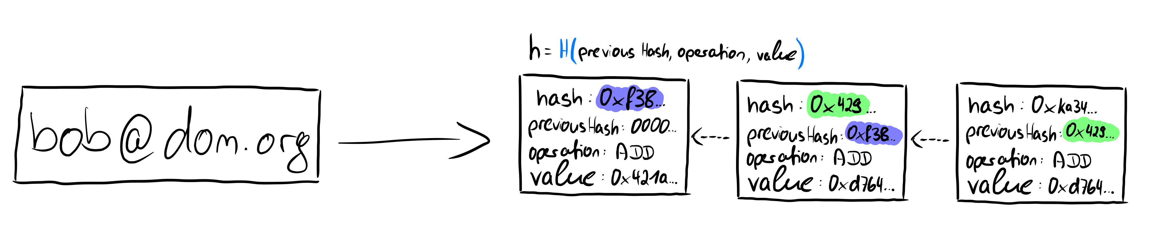
The image above shows the hash chain described in the paper. An identifier (e-mail address bob@dom.org) refers to this hash chain. The individual elements of the hash chain contain the operation performed (in the example of the first element, this must be an add operation to add the first public key) and the value that is added or revoked with the operation. In addition, each element contains a previous hash value, which makes the data structure a chain, since each element points to its predecessor. The first element of the hashchain has 0000... as its previous hash, which is comparable to a genesis block of a blockchain. Each element of the hashchain is uniquely identifiable by a hash value. This is created by giving all other values of the element into a hash function H: H(previous Hash, operation, value) = hash

Further, suppose that the first public key registered for bob@dom.org was legitimate.

To add new values, it is assumed that the first operation was done with good intentions. That is, it is assumed that Bob registered the Id bob@dom.org and that Oskar (in cryptography we often call the bad guys Oskar) didn't do so by impersonating Bob, otherwise all subsequent public keys would also be controlled by Oskar and not Bob, as other users of the dictionary would assume. Then Oskar is able to decrypt the symmetric keys that were intended for Bob to decrypt the messages and can view the secret documents.

We have now learned about the prerequisites, the basic ideas and the first data structure, the hashchain. Now we will get to know the second relevant data structure, which is of fundamental importance not only in this paper, but in cryptography as a whole: Merkle trees.

Merkle trees

Merkle trees are binary trees consisting of hash values. The actual values (texts, words, numbers, etc.) of the tree, the leaves, are hashed and these hashes are recursively hashed upwards in pairs, so that the next higher leaf node always consists of a hash generated by applying a hash function to the hashes of its two child nodes.

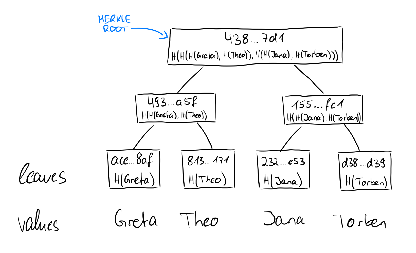
Here is an example of a Merkle tree where we store first names. We see that the values (in plain text at the bottom) are hashed and these hashes are then the leaves of the tree. The hashes of each two leaves are hashed again and combined to a parent node and so on until there is only one hash left: the root of the Merkle tree. Merkle trees have many nice features, which we will discuss in more detail later. For now, one of the important things to realize is that the merkle root depends on its contents starting with the leaves. Since the values are hashed and hash functions are collision resistant, the root computed in the example above has only this unique hash value (at least from a practical standpoint). We will understand the root of the Merkle tree later as a so-called cryptographic commitment and then go into more detail.

How Verdict uses Merkle Trees

We know that in Deimos, first names are not hashed and stored as in the above illustration, but rather public keys associated with email addresses. In Deimos, the Merkle trees are used as follows: We hash the email addresses with SHA256 and take the hash value of the last entry from the associated hashchain. Now we have two SHA256 hash values, consisting of - as the name suggests - 256 bits or the equivalent of 32 bytes.

One of the reasons and a conceivable problem is that for certain ids a very long hashchain exists because a lot of new keys have been added, while for other identifiers only a very short operation list exists. This is always somewhat inconvenient for subsequent proofs, as it means, at a minimum, that the length or size of the proofs are unpredictable and can vary widely. In this way, we turn the existing table which mapped ids to hashchains into a label-value pair with constant size.

However, the hash value of the leaves of the Merkle tree consists not only of the hashed label and the last hash of the hashchain (hereafter referred to as value), but also of two other things: an active flag and a next pointer. Our Transparency Dictionary theoretically has any number of columns, we can add very very very many email addresses with associated hashchains. To map this functionality in the Merkle tree that we manage in parallel with the dictionary is not very easy. Moreover, in our case, it is necessary that the existing two are powers, so 2, 4, 8, 16, 32... leaves are in the tree. This does not necessarily match with the number of entries in the dictionary and it is therefore possible that we have empty leaves. This is indicated by the active flag, which can take the values 1 (for an active leaf with matching entry in the dictionary) or 0 (for inactive leaf with null values). The next pointer is a reference to another leaf in the tree, we will see why we do this in a moment.

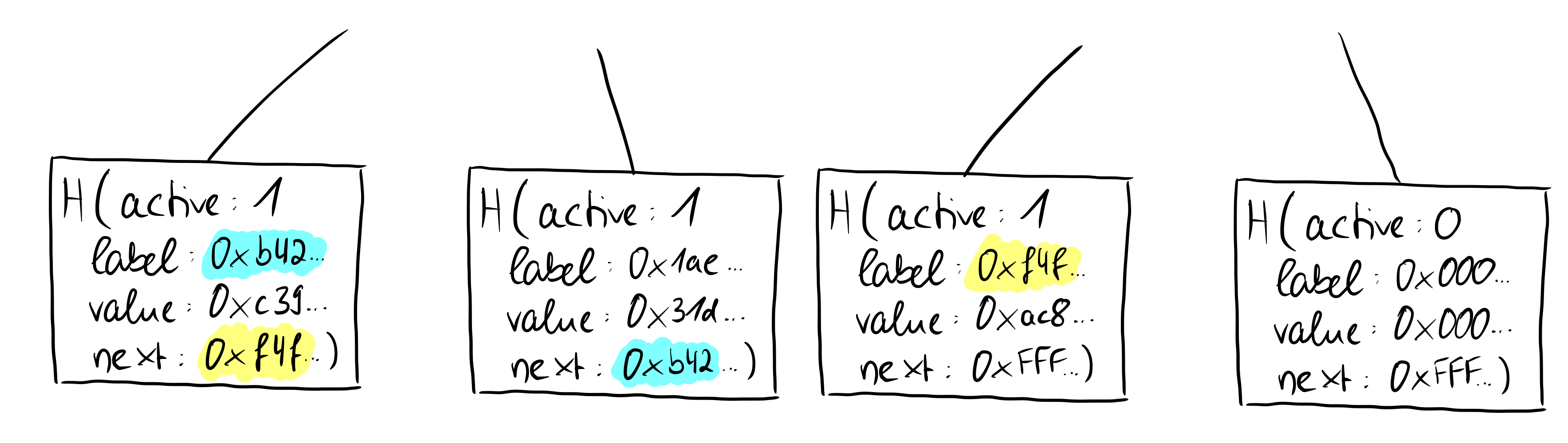
The picture illustrates several things about the Merkle Tree variant in the paper, the so-called indexed Merkle Trees:

• At which position the leaves are inserted in the tree is random, but they can still be sorted by their hexadecimal coding
• the next pointer points to the label with the next larger hexadecimal output or to a reserved label with a 64-fold repetition of the hexadecimal number "F" (or in bit notation 256x "1")
• inactive leaves have a fixed encoding

We take the last point as an opportunity to illustrate the possible elements of the leaves formally at a glance:
< active, label (hashed ID), value (last hash of the associated hashchain), next >
Inactive leaves are defined as follows:
< active = 0, label = 0x000...00, value = 0x000...00, next = label = 0xFFF...FF >

Rules for the "next"-Pointer

We take a closer look at the next pointer. We need two short, formal rules that we will need later to be able to save certain properties. These rules defined in the paper for the next-pointer are as follows:

1. the next-pointer of a node is either 0xFF...FFF, i.e. "the end", or
2. there is an active leaf to whose label the next pointer points and there is no other active leaf in between.

While the first rule is fairly self-explanatory, it may be worthwhile for us to visualize the second rule graphically.

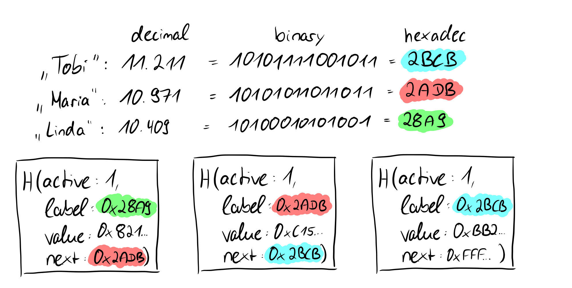
Simplified shown here are hash values for names (the output is of course much smaller than 256 bits, this is just for illustration). You can see that there is no other label value between the label values of "Linda" and "Maria". So for the leaves to the hashed values of "Linda" and "Maria" rule 2 can be applied, while for the hash value of "Tobi" rule 1 applies: the next pointer points to 0xFFF...FF.

What's next?

Great, now we not only understood the basic idea of Verdict, but also got to know the used data structures superficially. We've talked a lot about proving things before, we're approaching that now and getting to know the structures and ideas even better in that process.

• Let's proof something with knowledge
• Second thing to come
• Target in mind: zero knowledge proofs